Parameterisation of energy loss and total cross-section

Using the tabulated cross-section values of Seltzer and Berger together with the Migdal corrected Bethe-Heitler formula we have computed $\sigma (Z,T,k$_c)

and we have used these computed values as ``data points'' in the fitting procedure. Calculating the ``low energy'' ($T\le 10$ GeV) data we have applied the second Midgal correction to the results of Seltzer and Berger. We have chosen the parameterisations: $\sigma (Z,T,k$_c) ={Z(Z+ξ_σ)(T+m)²T(T+2m)}[ ln(T/k_c)]^αF_σ(Z,X,Y)&quad;(barn)

and $E$_Loss^brem(Z,T,k_c) ={Z(Z+ ξ_l)(T+m)²(T+2m)}[{k_cC_MT}]^βF_l(Z,X,Y) &quad;(GeV barn)

where m is the mass of the electron,

$X\; =\; ln(E/m),$	$Y\; =\; ln(v$σE/kc)
$X\; =\; ln(T/m),$	$Y\; =\; ln(k$c/vlE)	Lossbrem

with E=T+m. The constants $\xi$_σ, ξ_l, α, β, v_σ, v_l

are parameters to be fitted.

$C$M

$=$

$\{11+\{n\; r$0λ2(T+m)2πkc2}}

is the Midgal correction factor, with

$r$_o

classical electron radius;

$\lambda$

reduced electron Compton wavelength;

n

electron density in the medium.

$f(k/T)\; =\; \{\beta 2Z2\}k\{d\; \sigma dk\}=\; \{T(T+2m)(T+m)2Z2\}k\; \{d\; \sigma dk\}$

The functions $F$_i(Z,X,Y) ($i=\sigma ,l$ ) have the form $F$_i(Z,X,Y) = F_i0(X,Y)+ZF_i1(X,Y)

where $F$_ij(X,Y) are polynomials of the variables $X,Y$

$F$i0(X,Y)	$=$	$(C$1+C2X+...+C6X5)+(C7+C8X+...+C12X5)Y
		$+(C$13+C14X+...+ C18X5)Y2+...+(C31+C32X+...+C36X5)Y5
	$=$	$(C$1+C2X+...+C6X5)+(C7+C8X+...+C12X5)
		$+(C$37+C38X+...+C42X5)Y2+...+ (C55+C56X+...+C60X5)Y5
$F$i1(X,Y)	$=$	$(C$61+C62X+...+C65X4) +(C66+C67X+...+C70X4)Y
		$+(C$71+C72X+...+C75X4)Y2+...+(C81+C82X+...+C85X4) Y4
	$=$	$(C$61+C62X+...+C65X4) +(C66+C67X+...+C70X4)Y
		$+(C$86+C87X+...+C90X4)Y2+...+(C96+C97X+...+C100X4)Y4

$F$_ij(X,Y) denotes in fact a function constructed from two polynomials

$F$_ij(X,Y) =

$F$ijneg(X,Y)
$F$ijpos(X,Y)

$.$

where the polynomials $F$_ij fulfil the conditions

$F$_ij^neg(X,Y)_Y=0= F_ij^pos(X,Y)_Y=0&sp;( {F_ij^negY})_Y=0=( {P_ij^posY})_Y=0

We have computed 4000 ``data points'' in the range

_c≤T

and we have performed a least-squares fit to determine the parameters.

The values of the parameters ($\xi$_σ , $\alpha$ , $v$_σ , $C$_i for $\sigma$ and $\xi$_l , $\beta$ , $V$_l , C for $E$_Loss^brem ) can be found in the DATA statement within the functions GBRSGE and GBRELE which compute the formula () and () respectively.

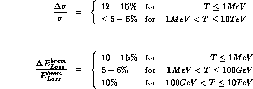
The errors of the parameterisations () and () can be estimated as

We have performed a fit to the ``data'' without the Midgal corrections, too. In this case we used the data of Seltzer and Berger without any correction for $T\; \le 10$ GeV and we used the Bethe-Heitler cross-section for $T\; \ge 10$ GeV. The parameterised forms of the cross-section and energy loss are the same as they were in the first fit (i.e. () and ()), only the numerical values of the parameters have changed. These values are in DATA statements in the functions GBRSGE and GBRELE and this second kind of parameterisation can be activated using the PATCHY switch +USE,BETHE. (The two parameterisations give different results for high electron energy.)

The energy loss due to soft photon bremsstrahlung is tabulated at initialisation time as a function of the medium and of the energy by routine GBRELA (see JMATE data structure).

The mean free path for discrete bremsstrahlung is tabuled at initialisation time as a function of the medium and of the energy by routine GBRSGA (see JMATE data structure).